pytorch搭建CNN网络实现MNIST数据集的图像分类

前言

最近趁着学校暑期实验室实践进了实验室，跟着导师参与一些简单的项目，学习一些知识，积累一点经验，由于参与的项目是与深度学习有关的，所以也算入了深度学习的坑，开始学一点基础知识，这篇文章就算是深度学习之旅的开端吧，搭建了第一个CNN网络，做出了第一个图像分类器，最然只是最简单的东西，但是也算是入了门，相信以后会学到更多的更深入的东西，特意在此记录一下做出的成果。

顺便一提，我在GitHub上新建了一个repo，会陆陆续续把自己学习深度学习过程中做的一些东西和一些经验分享上去（虽然现在还很空荡），欢迎大家star和fork。链接在此：begin-deep-learning

代码部分

代码各部分都做了一定的注释，所以这里就不再一一解释，可能之后还会出jupyter notebook版本，会加上更加详尽的注释，可能会更加清晰。

import torch
import torchvision
import torchvision.transforms as transforms
import matplotlib.pyplot as plt
import torch.nn as nn
import torch.nn.functional as F
import torch.optim as optim
from torch.utils.data import DataLoader
from torch.autograd import Variable

# 加载mnist数据集
EPOCH = 5
BATCH_SIZE = 100
LR = 0.001
DEVICE = torch.device('cuda' if torch.cuda.is_available() else 'cpu')
'''
transform=torchvision.transforms.Compose([
                               torchvision.transforms.ToTensor(),
                               torchvision.transforms.Normalize(
                                 (0.1307,), (0.3081,))
                             ])
     '''
train_data = torchvision.datasets.MNIST( # train_set
    root='./data/',
    train=True,
    transform=transforms.ToTensor(),
    download=False # 首次使用设为True来下载数据集，之后设为False
)
test_data = torchvision.datasets.MNIST( # test_set
    root='./data/',
    train=False,
    transform=transforms.ToTensor(),
    download=False
)
train_loader = DataLoader(
    dataset=train_data,
    batch_size=BATCH_SIZE,
    shuffle=True
)
test_loader = DataLoader(
    dataset=test_data,
    batch_size=BATCH_SIZE,
    shuffle=False
)

'''
# 查看数据（可视化数据）
def datashow(train_loader):
    images, label = next(iter(train_loader))
    images_example = torchvision.utils.make_grid(images)
    images_example = images_example.numpy().transpose(1,2,0) # 将图像的通道值置换到最后的维度，符合图像的格式
    mean = [0.5,0.5,0.5]
    std = [0.5,0.5,0.5]
    images_example = images_example * std + mean
    print(labels)
    plt.imshow(images_example )
    plt.show()
'''

# 模型搭建（参考pytorch官网）
class Net(nn.Module):

    def __init__(self):
        super(Net, self).__init__()
        # 1 input image channel, 6 output channels, 5x5 square convolution
        # kernel
        self.conv1 = nn.Conv2d(1, 6, 3, 1, 2)
        self.conv2 = nn.Conv2d(6, 16, 5)
        # an affine operation: y = Wx + b
        self.fc1 = nn.Linear(16 * 5 * 5, 120)
        self.fc2 = nn.Linear(120, 84)
        self.fc3 = nn.Linear(84, 10)

    def forward(self, x):
        # Max pooling over a (2, 2) window
        x = F.max_pool2d(F.relu(self.conv1(x)), (2, 2))
        # If the size is a square you can only specify a single number
        x = F.max_pool2d(F.relu(self.conv2(x)), 2)
        x = x.view(-1, self.num_flat_features(x))
        x = F.relu(self.fc1(x))
        x = F.relu(self.fc2(x))
        x = self.fc3(x)
        return x

    def num_flat_features(self, x):
        size = x.size()[1:]  # all dimensions except the batch dimension
        num_features = 1
        for s in size:
            num_features *= s
        return num_features

net = Net().to(device=DEVICE)
# 定义损失函数和优化函数
criterion = nn.CrossEntropyLoss()
optimizer = optim.Adam(net.parameters(), lr=LR)


train_counter = []
train_losses = []
train_accs = []
test_losses = []
test_counter = [i*len(train_loader.dataset) for i in range(EPOCH)]

# 模型训练
def train(epoch):
    #for epoch in range(EPOCH):  # loop over the dataset multiple times

    #train_loss = 0.0
    for i, data in enumerate(train_loader, 0):
        # get the inputs
        inputs, labels = data
        inputs, labels = Variable(inputs).cuda(), Variable(labels).cuda()

        # zero the parameter gradients
        optimizer.zero_grad()

        # forward + backward + optimize
        outputs = net(inputs) # 将数据传入网络进行前向运算
        loss = criterion(outputs, labels) # 得到损失函数
        loss.backward() # 反向传播
        optimizer.step() # 通过梯度做一步参数更新

        # print statistics
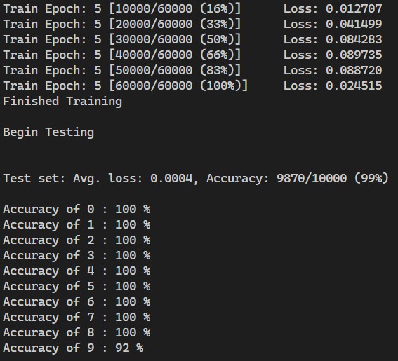
        if i % 100 == 99:
            print('Train Epoch: {} [{}/{} ({:.0f}%)]\tLoss: {:.6f}'.format(
                epoch, (i+1) * len(inputs), len(train_loader.dataset),
                100. * i / len(train_loader), loss.item()))
        train_losses.append(loss.item())
        train_counter.append((i*BATCH_SIZE) + ((epoch-1)*len(train_loader.dataset)))

        correct = 0
        total = 0
        _, predicted = torch.max(outputs.data, 1)
        total = labels.size(0)# labels 的长度
        correct = (predicted == labels).sum().item() # 预测正确的数目
        train_accs.append(100*correct/total)

    print('Finished Training')

# 模型测试
def test():
    print('\n'+"Begin Testing"+'\n')
    net.eval()
    correct = 0
    total = 0
    test_loss = 0
    with torch.no_grad():
        for data in test_loader:
            images, labels = data
            images, labels = Variable(images).cuda(), Variable(labels).cuda()
            outputs = net(images)
            loss = criterion(outputs, labels) # 得到损失函数
            test_loss += loss.item()
            _, predicted = torch.max(outputs.data, 1)
            total += labels.size(0)
            correct += (predicted == labels).sum().item()
    test_loss /= total
    test_losses.append(test_loss)
    print('Test set: Avg. loss: {:.4f}, Accuracy: {}/{} ({:.0f}%)\n'.format(
    test_loss, correct, total,
    100. * correct / total))

    class_correct = list(0. for i in range(10))
    class_total = list(0. for i in range(10))
    with torch.no_grad():
        for data in test_loader:
            images, labels = data
            images, labels = Variable(images).cuda(), Variable(labels).cuda()
            outputs = net(images)
            _, predicted = torch.max(outputs, 1)
            c = (predicted == labels).squeeze()
            for i in range(4):
                label = labels[i]
                class_correct[label] += c[i].item()
                class_total[label] += 1
    for i in range(10):
        print('Accuracy of %s : %2d %%' % (i, 100 * class_correct[i] / class_total[i]))


for epoch in range(1, EPOCH + 1):
    train(epoch)
    test()
fig = plt.figure()
plt.plot(train_counter, train_losses, color='blue')
plt.scatter(test_counter, test_losses, color='red')
plt.legend(['Train Loss', 'Test Loss'], loc='upper right')
plt.xlabel('epoch')
plt.ylabel('loss')
plt.show()

结果展示

结果图如下：

自行修改EPOCH和LR可以得到不同的结果，代码中为我调好的参数，可以看出只需要训练四轮左右就可以达到99%的准确率。